Simple Database Implementation (Optimization)

Lab Assignment Part 3. From MIT 6.830. See http://dsg.csail.mit.edu/6.830/

Introduction

This article will focus on the query optimization of the database, including an estimation framework and a cost-based optimizer called Selinger.

Control Flow

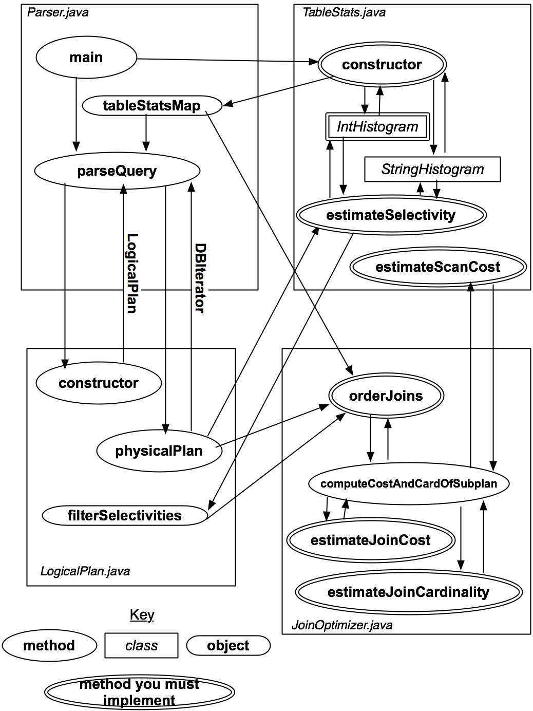
This diagram is from the class page.
Parser.java: It is responsible for parsing the query. It will pass itself to TableStats.java to analysize some details of the query, and pass the query to the LogicalPlan.java to build a physicalPlan.
TableStats.java: It is responsible for estimating selectivity and scancost of the query by building a histogram.
LogicalPlan.java: It is responsible for creating a physical plan of a query, namely converting a join statement to a physical iterator on tuples.
JoinOptimizer.java: It is the main optimizer class. The OrderJoins method will receive all data needed and use dynamic programming to optimize the query.

Reflection

Theory

Plan Cost

Given a join plan p = t1 join t2 join ... join tn, its cost can be expressed as:

scancost(t1) + scancost(t2) + joincost(t1 join t2) + 
scancost(t3) + joincost((t1 join t2) join t3) + 
...

Here, scancost(t1) is the I/O cost of scanning table t1, we can simply regard it as the number of pages in t1. joincost(t1 join t2) is the CPU cost to join t1 and t2. As I used nested loops joins in the previous lab, I can use the following formular to calculate that:

joincost(t1 join t2) = scancost(t1) + ntups(t1) * scancost(t2) // IO cost
                        + ntups(t1) * ntups(t2) // CPU cost

Optimizer

Optimizer is the most complex problem in SQL Database. Normally, there are two large categories: Rule-Based Optimizer and Cost-Based Optimizer. Rule-Based Optimizer will equivalently change the tree representation of the specified list of joins to make it more efficient. For example, pushing selection down in the tree will result in better execution plans in any situations. Cost-Based Optimizer will apply algebraic laws, start from partial plans, build more complete plans, until estimated cost is minimal. Dynamic programming is often used to reduce the number of partial plans. Here is a pseducode of Selinger used in SimpleDB:

j = set of join nodes
for (i in 1...|j|):
     for s in {all length i subsets of j}
            bestPlan = {}
       for s' in {all length d-1 subsets of s}
            subplan = optjoin(s')
            plan = best way to join (s-s') to subplan
            if (cost(plan) < cost(bestPlan))
               bestPlan = plan
      optjoin(s) = bestPlan
 return optjoin(j)

Design

In order to better analyze queries, simpleDB created several classes to help parse them. For example, a query:

SELECT A.C, A.D
FROM A
LEFT JOIN B ON A.C == B.C
WHERE A.D > 0

LogicalSelectListNode will have the information in the SELECT list, namely A.C and A.D.
LogicalScanNode will have the information in the FROM list, namely table A.
LogicalJoinNode will have the information in the JOIN list, namely table A, B and field C. LogicalFilterNode will have the information in the WHERE list, namely A.D, 0, and predicate >.
These classes can be sent to different places and complete various analysis.

Another design I’d like to talk about is when estimating ntups for a table with one or more selection predicates over it (See theory part above for why we need to estimate ntup). We can build a histogram for every attribute in the table. First, scan the table to get the minimum and maximum values. Then, divide the histogram into a fixed number of buckets, with each bucket representing the number of records in the range of the domain of the attribute of the histogram. For example, a field f ranges from 1 to 100, and there are 10 buckets. Bucket 1 contain the number of records between 1 and 10, and so on.

• simpledb